Background

A notable feature of the Baltic hydrography is the presence of a generally east-west and north-south salinity gradient and salinity stratification of the water column, as you have identified in case study 1. The complex hydrographic regime of the Baltic, its short, but dynamic evolution, and the human intervention resulted in the biota consisting of species of various origins and environmental tolerances that have immigrated or been artificially introduced to the area over the relatively recent history of the system. These are marine and freshwater species, migratory species, and glacial relicts. Representatives of these categories have different environmental preferences as well as tolerances and the composition of communities therefore varies greatly in different regions of the Baltic Sea, depending primarily on salinity, water temperature, oxygen content, and nutrient concentrations. Regional climate change models predict an increase in temperature and a decrease in salinity but a high uncertainty remains about the impact of climate change on fish stocks.

In this case study, we will investigate the winter distribution (1. quarter of the year: Jan- March) of the 8 most abundant fish species in 2015 (Fig.1) using the BITS monitoring data. Since 2001, the Baltic International Trawl Surveys (BITS) has been carried out with a harmonized sampling scheme and standard gear to sample the demersal fish community in the Baltic Sea. This sampling scheme consists of trawl hauls with a duration of 30 minutes, carried at a speed of 3 knots with a demersal otter trawl gear (TV3 with mesh size of 520 or 930 mm). The gear is best suited for sampling demersal fish such as gadoids and flatfish. The dataset was downloaded from the ICES Database for Trawl Surveys (DATRAS; http://datras.ices.dk/ Home/Default.aspx; data downloaded on the 20th of Dec 2017).

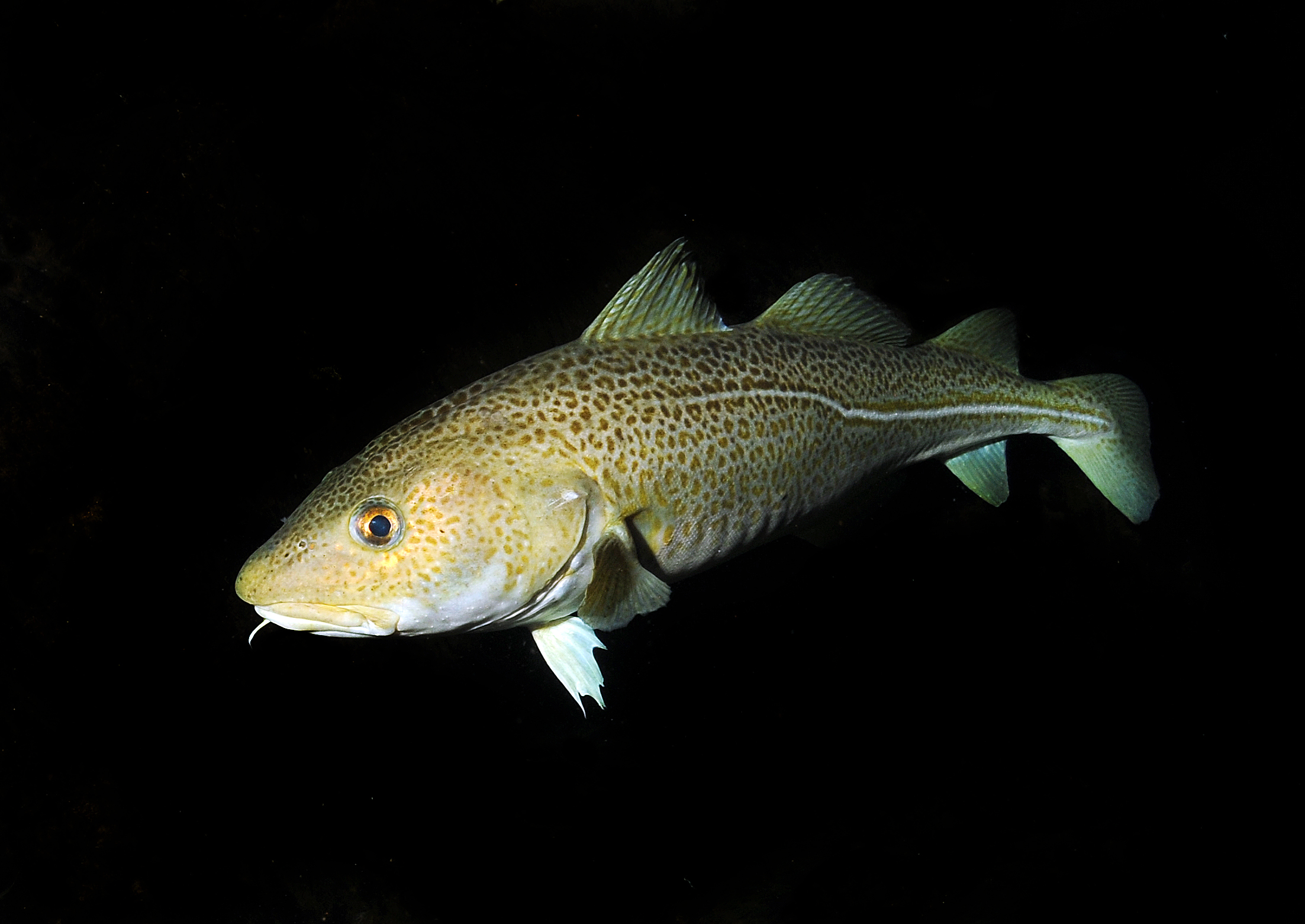
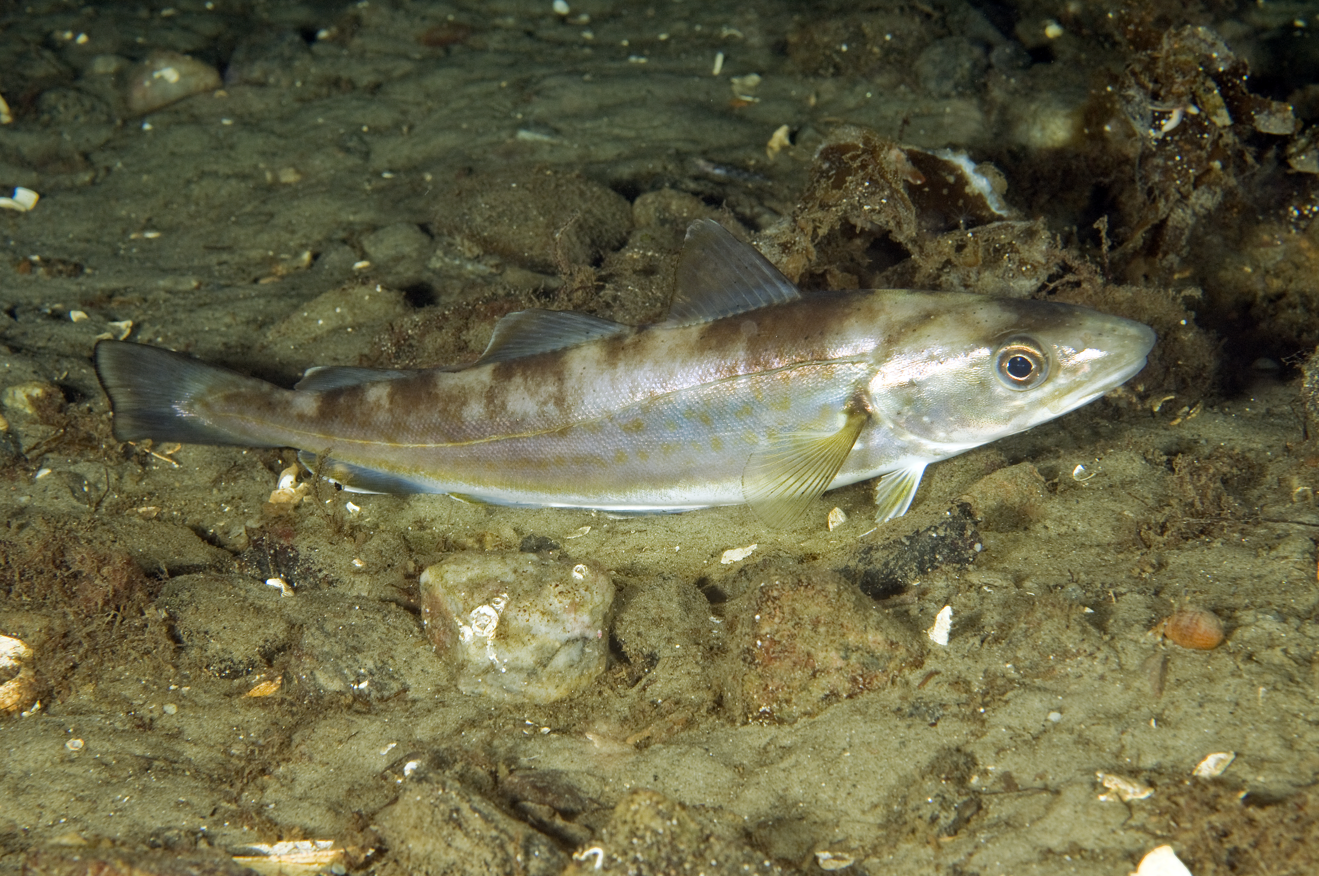
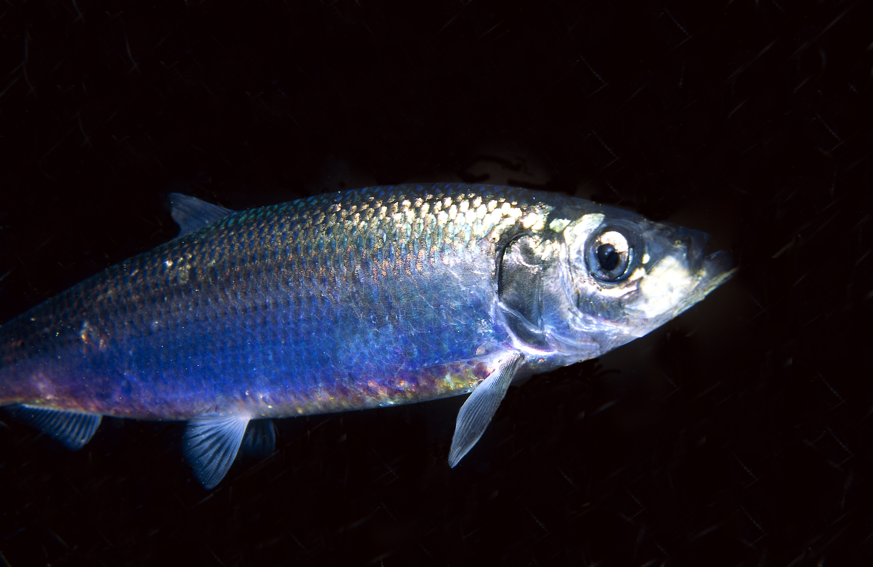
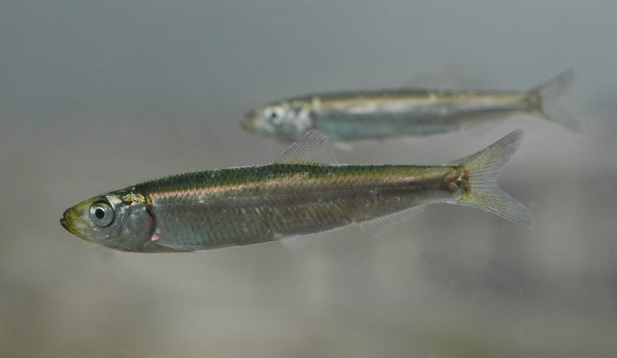
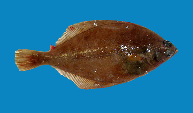
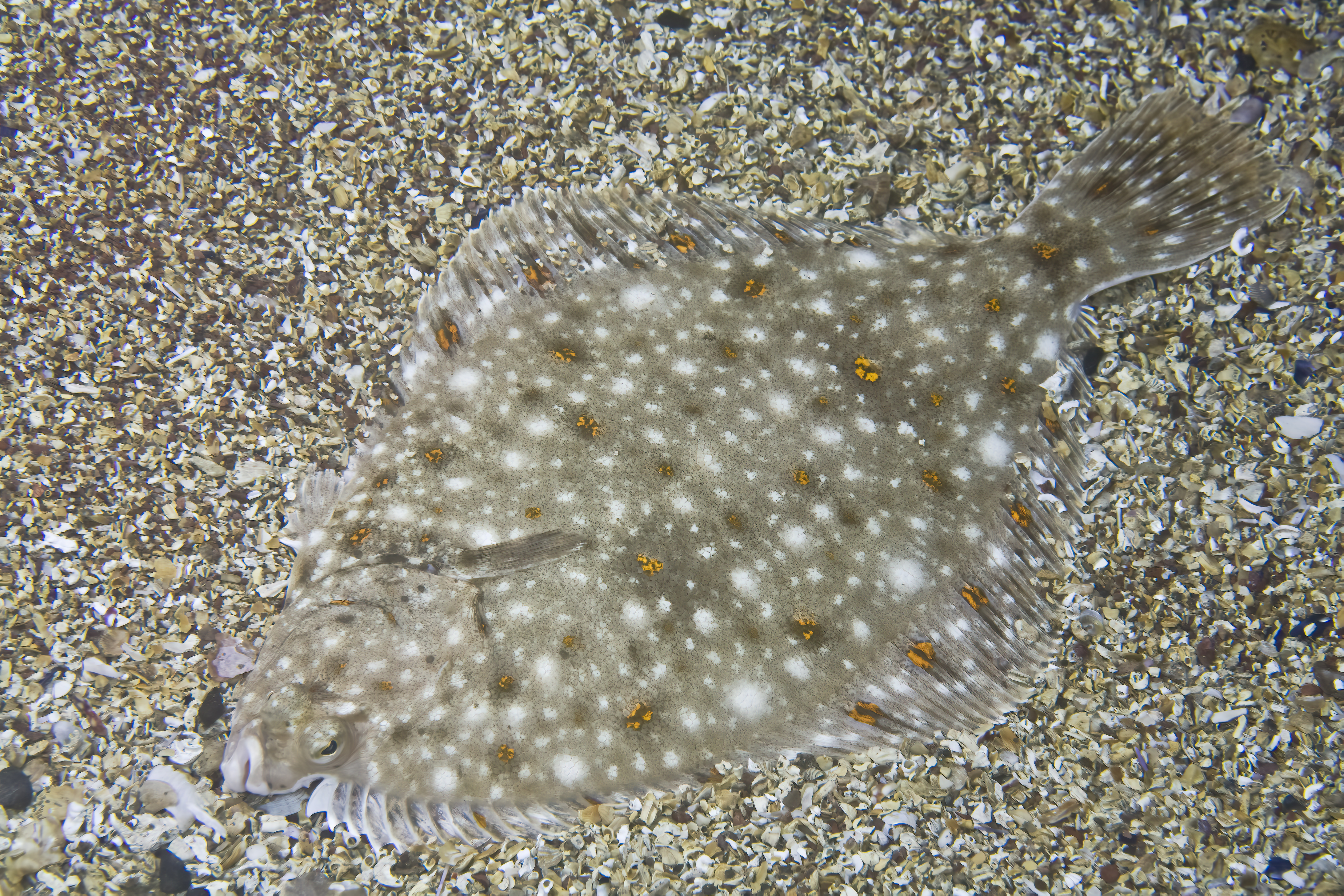
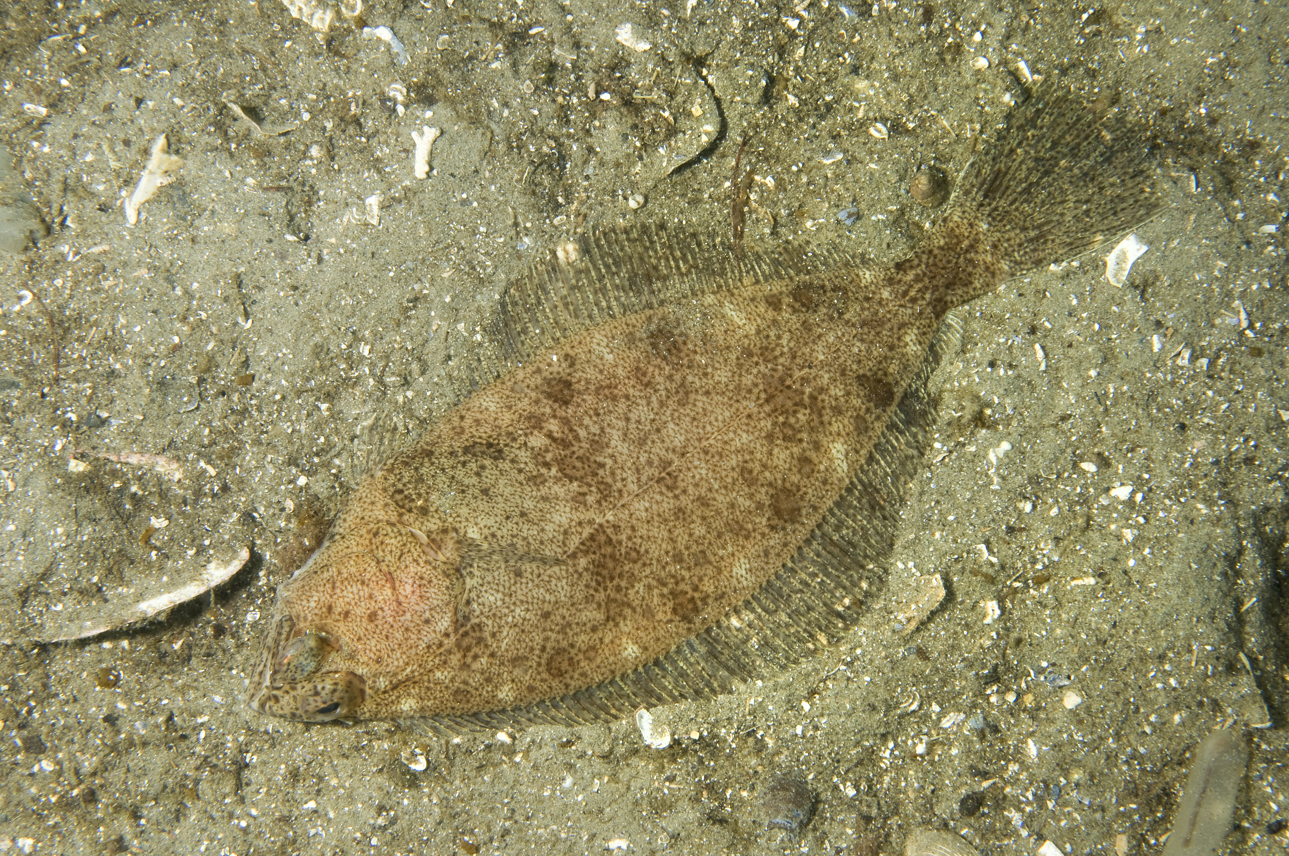
Fig 1. Upper row showing from left to right: Atlantic cod (© R. Svensen), whiting (© R.S.), Atlantic herring (© R.S.), European sprat (© R.S.); lower row showing: European flounder (© K.I. Stergiou), Common dab (© G.-P. Zauke), European plaice (© J. Greenfield), American plaice (© R.S.). Image courtesy of the above photographers at fishbase.org and uwphoto.com (R. Svensen).

The data set contains also salinity and temperature values for every haul. This data stems from the oceanographic database provided by ICES, which was interpolated to generate predicted winter values for the location of the hauls taken.

load("data/data_case_study_2.R")
str(cpue15)

## Classes 'tbl_df', 'tbl' and 'data.frame':    1419 obs. of  12 variables:
##  $ year          : int  2015 2015 2015 2015 2015 2015 2015 2015 2015 2015 ...
##  $ lat           : num  54.1 54.1 54.1 54.1 54.1 ...
##  $ long          : num  11.2 11.2 11.2 11.2 11.2 ...
##  $ depth         : int  24 24 24 24 24 24 24 18 18 18 ...
##  $ area          : int  22 22 22 22 22 22 22 22 22 22 ...
##  $ subarea       : int  9 9 9 9 9 9 9 8 8 8 ...
##  $ gear          : chr  "TVS" "TVS" "TVS" "TVS" ...
##  $ species       : chr  "Clupea harengus" "Gadus morhua" "Limanda limanda" "Merlangius merlangus" ...
##  $ cpue_total    : num  340 859 262 744 96 ...
##  $ cpue_total_log: num  5.83 6.76 5.57 6.61 4.56 ...
##  $ temp_pred     : num  4.04 4.04 4.04 4.04 4.04 ...
##  $ sal_pred      : num  23.3 23.3 23.3 23.3 23.3 ...

The tibble contains information for each haul: the year, the coordinates, the respective ICES subdision and subarea, the gear type (“TVS” = small trawl type of 520 meshes, “TVL” = large trawl of 930 meshes), the 8 species, the total CPUE and its log-transformed value, and the interpolated temperature and salinity values. To avoid the problem of zero-inflation in your models, all zero values have been filtered out!

Your task

Study the effects of latitude, longitude, depth and hydrography on the number of caught fish - in areas where the species are present (since we use presence-only data). You can also download the data and do the data wrangling yourself and compare with the one provided here (although it will not contain the salinity and temperature then). Some instructions for this are below.