Data Analysis with R
18 - Iteration 2 (purrr and the map family)
Saskia A. Otto
Postdoctoral Researcher
Functional programming
Loops
forloops are not as important in R as they are in other languages because R is a functional programming language.- It is possible to wrap up
forloops in a function, and call that function instead of using the for loop directly.
Consider (again) this simple data frame:

Functional programming with purrr
- As you have seen, passing a function to another function is extremely handy, reduces potential bugs (much less code and copy and pasting), and makes it easy to generalise
- The apply family of functions in base R (
apply(),lapply(),sapply(),vapply(),tapply(),mapply()) does exactly that: Thes functions act on an input list, vector, dataframe, matrix or array, and apply a named function with one or several optional arguments. - The map family of functions provided by the tidyverse packages purrr operates similar but can be faster (all functions written in C++), is more consistent, well integrated in the tidyverse concept and easier to learn.
- purrr provides in addition many more useful functions for handling lists; to have an overview of available functions see the cheatsheet
The most basic function: map()

The most basic function: map()
Using our previous example:
set.seed(1)
df <- data.frame(
  x = rnorm(20),
  y = rnorm(20),
  z = rnorm(20)
)
map() always preserves the list names.
map(df, mean)
## $x
## [1] 0.1905239
##
## $y
## [1] -0.006471519
##
## $z
## [1] 0.1387968
# You can also use the pipe operator
df %>% map(median)
The ... argument
Here you specify all other arguments which can be specified in the function used:
map(df, quantile, probs = c(0,0.5,1.0) )
## $x
##         0%        50%       100%
## -2.2146999  0.3596755  1.5952808
##
## $y
##          0%         50%        100%
## -1.98935170 -0.05496689  1.35867955
##
## $z
##         0%        50%       100%
## -1.1293631  0.1143867  1.9803999
Other types of output than a list
map_lgl()→ returns a logical vectormap_int()→ returns an integer vectormap_dbl()→ returns a double vectormap_chr()→ returns a character vector
The length of the returned vector and .x are always the same!
To get the means of x, y and z as vector replace map() with the appropriate function:
map_dbl(df, mean)
##            x            y            z
##  0.190523876 -0.006471519  0.138796773
Note: :
`map_dbl()` returns a named vector based on the original list names!Other types of output than a list
You can always generate a vector of a more general data type but not the opposite
map_int(df, mean)
## Error: Can't coerce element 1 from a double to a integer
map_chr(df, mean)
##           x           y           z
##  "0.190524" "-0.006472"  "0.138797"
Your turn...
Task: Explore the data
Load the following R datafile, which contains the list groundsharks:
load("data/fishbase_sharks.R")
ls()
## [1] "groundsharks"
This list contains data for 284 groundshark species (Carcharhiniformes, the largest order of sharks) downloaded from fishbase. The list has a hierarchical structure with one list per species containing individual sublists for each information.
Task: Explore the data
Answer the following questions
- How many elements are in groundsharks?
- What is the first species listed in groundsharks? What information is given for this species?
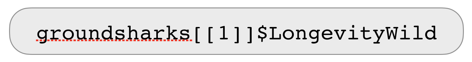
- What is the difference between groundsharks[1] and groundsharks[[1]]?
(Answers are on the next slide)
length(groundsharks[[1]])
## [1] 99
names(groundsharks[[1]])
##  [1] "sciname"              "Genus"                "Species"
##  [4] "SpeciesRefNo"         "Author"               "FBname"
##  [7] "PicPreferredName"     "PicPreferredNameM"    "PicPreferredNameF"
## [10] "PicPreferredNameJ"    "FamCode"              "Subfamily"
## [13] "GenCode"              "SubGenCode"           "BodyShapeI"
## [16] "Source"               "AuthorRef"            "Remark"
## [19] "TaxIssue"             "Fresh"                "Brack"
## [22] "Saltwater"            "DemersPelag"          "AnaCat"
## [25] "MigratRef"            "DepthRangeShallow"    "DepthRangeDeep"
## [28] "DepthRangeRef"        "DepthRangeComShallow" "DepthRangeComDeep"
## [31] "DepthComRef"          "LongevityWild"        "LongevityWildRef"
## [34] "LongevityCaptive"     "LongevityCapRef"      "Vulnerability"
## [37] "Length"               "LTypeMaxM"            "LengthFemale"
## [40] "LTypeMaxF"            "MaxLengthRef"         "CommonLength"
## [43] "LTypeComM"            "CommonLengthF"        "LTypeComF"
## [46] "CommonLengthRef"      "Weight"               "WeightFemale"
## [49] "MaxWeightRef"         "Pic"                  "PictureFemale"
## [52] "LarvaPic"             "EggPic"               "ImportanceRef"
## [55] "Importance"           "PriceCateg"           "PriceReliability"
## [58] "Remarks7"             "LandingStatistics"    "Landings"
## [61] "MainCatchingMethod"   "II"                   "MSeines"
## [64] "MGillnets"            "MCastnets"            "MTraps"
## [67] "MSpears"              "MTrawls"              "MDredges"
## [70] "MLiftnets"            "MHooksLines"          "MOther"
## [73] "UsedforAquaculture"   "LifeCycle"            "AquacultureRef"
## [76] "UsedasBait"           "BaitRef"              "Aquarium"
## [79] "AquariumFishII"       "AquariumRef"          "GameFish"
## [82] "GameRef"              "Dangerous"            "DangerousRef"
## [85] "Electrogenic"         "ElectroRef"           "Complete"
## [88] "GoogleImage"          "Profile"              "PD50"
## [91] "Emblematic"           "Entered"              "DateEntered"
## [94] "Modified"             "DateModified"         "Expert"
## [97] "DateChecked"          "TS"                   "SpecCode"
Quiz 1: What is the longevity of each species in the wild?
(this information is stored in LongevityWild)
STRATEGY
- Do it for one element
- Turn it into a recipe
- Use
map()to do it for all elements
1. What is the longevity for the blacknose shark (the first species in the list)?
- Solve the problem for one element
2. Turn it into a receipe
- Make it a formula
- Use .x as a pronoun
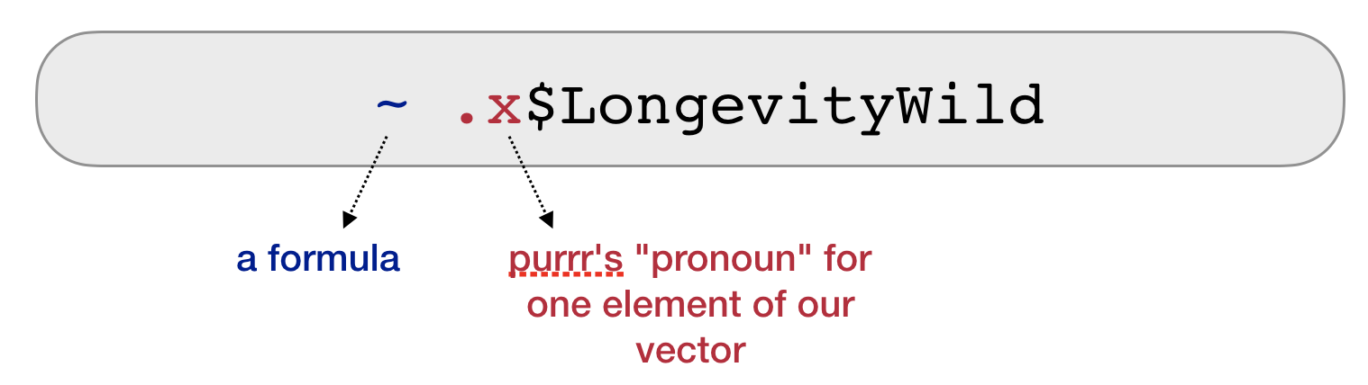
3. Do it for all elements
- Your recipe is the second argument to map
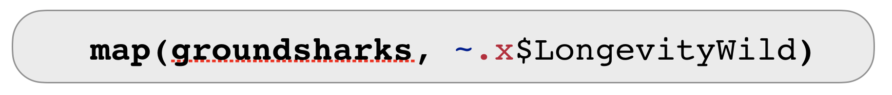
Quiz 2: What is the mean longevity in the wild across all shark and ray species?
Solution: What is the mean longevity in the wild across all shark and ray species?
Applying a mean to a list is difficult ➔ use map_dbl() to get a vector returned:
map_dbl(groundsharks, ~ .x$LongevityWild) %>% mean(na.rm = TRUE)
## [1] 20.125
Ways of specifying .f
.f can be a formula
map_int(groundsharks, ~ length(.x)) %>% head()
## [1] 99 99 99 99 99 99
map_chr(groundsharks, ~ .x[["FBname"]]) %>% head()
## [1] "Blacknose shark"      "Silvertip shark"      "Bignose shark"
## [4] "Graceful shark"       "Blacktail reef shark" "Pigeye shark"
map_chr(groundsharks, ~ .x$FBname) %>% head()
## [1] "Blacknose shark"      "Silvertip shark"      "Bignose shark"
## [4] "Graceful shark"       "Blacktail reef shark" "Pigeye shark"
.f can be a string or integer
- For each element, extract the named or numbered element.

map_chr(groundsharks, .f = "FBname")

# use an integer to select elements by position:
map(groundsharks, 97)
.f can be a function
- For each element, extract the named or numbered element.

map(.x = df, .f = mean, na.rm = TRUE)
map(.x = df, ~ mean(.x, na.rm = TRUE))
Combining map functions
How long is each species name?
# 1. Extract the scientific species name
char_species <- map(groundsharks, "sciname")
# 2. Get the length of the name (= number of characters)
map_int(char_species, str_length) %>% head()
## [1] 22 27 20 29 26 24
# Piping both map functions
map(groundsharks, "sciname") %>% map_int(str_length) %>% head()
## [1] 22 27 20 29 26 24
# Now in one go
map_int(groundsharks, ~ str_length(.x[["sciname"]])) %>% head()
## [1] 22 27 20 29 26 24
set_names()
is a useful function for extracting information from sublists and using this to set the names of another list.
- Example: Get the corresponding scientific name to each length value:
# First extract the length values ...
map_dbl(groundsharks, .f = "Length") %>%
  # ...and give it the names from sciname
  set_names(map_chr(groundsharks, .f = "sciname")) %>% head()
##        Carcharhinus acronotus   Carcharhinus albimarginatus
##                           200                           300
##          Carcharhinus altimus Carcharhinus amblyrhynchoides
##                           300                           161
##    Carcharhinus amblyrhynchos      Carcharhinus amboinensis
##                           255                           280
Your turn...
Quiz 3: Extract more information from 'groundsharks'
- Which species has the highest weight?
- Which species has the lowest vulnerability score?
- Which species swims deepest?
- Which species do we know the least about (i.e. have the most NA entries)?
Solutions 1 + 2
# Species with the highest weight
map_dbl(groundsharks, .f = "Weight") %>%
  set_names(map_chr(groundsharks, .f = "FBname")) %>%
  sort() %>% tail(n = 1)
## Tiger shark
##      807400
# Species with the lowest vulnerability score
map_dbl(groundsharks, .f = "Vulnerability") %>%
  set_names(map_chr(groundsharks, .f = "FBname")) %>%
  sort() %>% head(n = 1)
## Pygmy ribbontail catshark
##                     12.55
Solutions 3 + 4
# Species that swims deepest
map_dbl(groundsharks, .f = "DepthRangeDeep") %>%
  set_names(map_chr(groundsharks, .f = "FBname")) %>%
  sort() %>% tail(n = 1)
## Silky shark
##        4000
# Species we know least about
map_int(groundsharks, ~ sum(is.na(.x))) %>%
  set_names(map_chr(groundsharks, .f = "sciname")) %>%
  sort() %>% tail(n = 1)
## Haploblepharus kistnasamyi
##                         60
Other iteration functions
Mapping over 2 arguments: map2()

map2()applies a function to PAIRS of elements from two lists, vectors, etc.- to get a vector returned:
map2_lgl(),map2_int(),map2_dbl(),map2_chr()
Mapping over 2 arguments: map2()
map2(.x = c("a","b","c"), .y = c(1,2,3), .f = rep)
## [[1]]
## [1] "a"
##
## [[2]]
## [1] "b" "b"
##
## [[3]]
## [1] "c" "c" "c"
Mapping over multiple arguments: pmap()

pmap()applies a function to GROUPS of elements FROM a LIST of lists, vectors, etc.- NO corresponding
pmap_lgl(),pmap_int(), etc.
Mapping over multiple arguments: pmap()
Example: sample from these 3 vectors 2, 10, or 5 times with or without replacement
arg_list <- list(x = list(a = 1:10, b = 1:5, c = 1:20), size = c(2, 10, 5),
  repl = c(FALSE, TRUE, FALSE))
pmap(.l = arg_list, .f = sample)
## $a
## [1] 10  5
##
## $b
##  [1] 3 1 4 3 3 2 2 3 3 1
##
## $c
## [1]  1 13 17 11  9
One more step in complexity:
Invoking different functions with invoke_map()
As well as varying the arguments to the function you might also vary the function itself. Example: Apply the mean, median and sd to a single vector or to a list:
# Single vector
invoke_map(.f = list(mean, median, sd),
  x = 1:10)
## [[1]]
## [1] 5.5
##
## [[2]]
## [1] 5.5
##
## [[3]]
## [1] 3.02765
# List
params <- list(alist(x= 1:15),
  list(x=200:400), list(x=1:4))

invoke_map_dbl(.f = list(mean, median,
  sd), .x = params)
## [1] 8.000000 300.000000 1.290994
Other mapping functions
invoke(),lmap(),imap(),walk(),walk2(),pwalk()for side effects (returns input invisibly)
Your turn...
Lets go back to the exercise in the previous lecture on loops:
Write a function to fit a linear model to each data.frame (column x vs column y) and plot the slopes as histogram. You can use multiple files ("ex_final_multifile_1.csv", "ex_final_multifile_2.csv", ...) or a single file ("ex_final_one_file.csv") to solve this....
Lets tackle this task with purrr:
- import "dummyfile_1.csv" - "dummyfile_100.csv" so that you have one data list
- apply the linear model to each dataframe using one of the
mapfunctions - extract the slopes and create a histogram
Solution
# 1. Import
files <- str_c("data/functions/dummyfile_", 1:100, ".csv")
data_list <- map(files, read_csv)
# Lets add a column with the name of the file
data_list <- map2(.x = data_list, .y = as.character(1:100), ~ mutate(.x, dataset = .y))

# 2. Apply linear models, extract slope and plot the histogram
map(data_list, ~ lm(y ~ x, data = .x)) %>%
  map_dbl(~ coef(.x)[2]) %>%
  hist(main = "Distributions of slopes")

purrr and list-columns
list-columns
- Data frames are a extremely handy data structure for data analysis:
- they are more clearly structured than a list (similar to a matrix)
- but they can contain different data types (which the matrix cannot)
- being a hybrid between a list and matrix allows a very flexible usage, e.g. dataframes can be indexed like a list or a matrixs
- We typically regard data frames a container for several atomic vectors of the same or different data type with a common length.
- But data frames are even more flexible! They can contain all vector types, that includes list (recall: atomic vectors and lists represent together vectors!)
- Such list in a data frame are called list-columns
- You can even store individual ggplot objects in list-columns!
list-columns
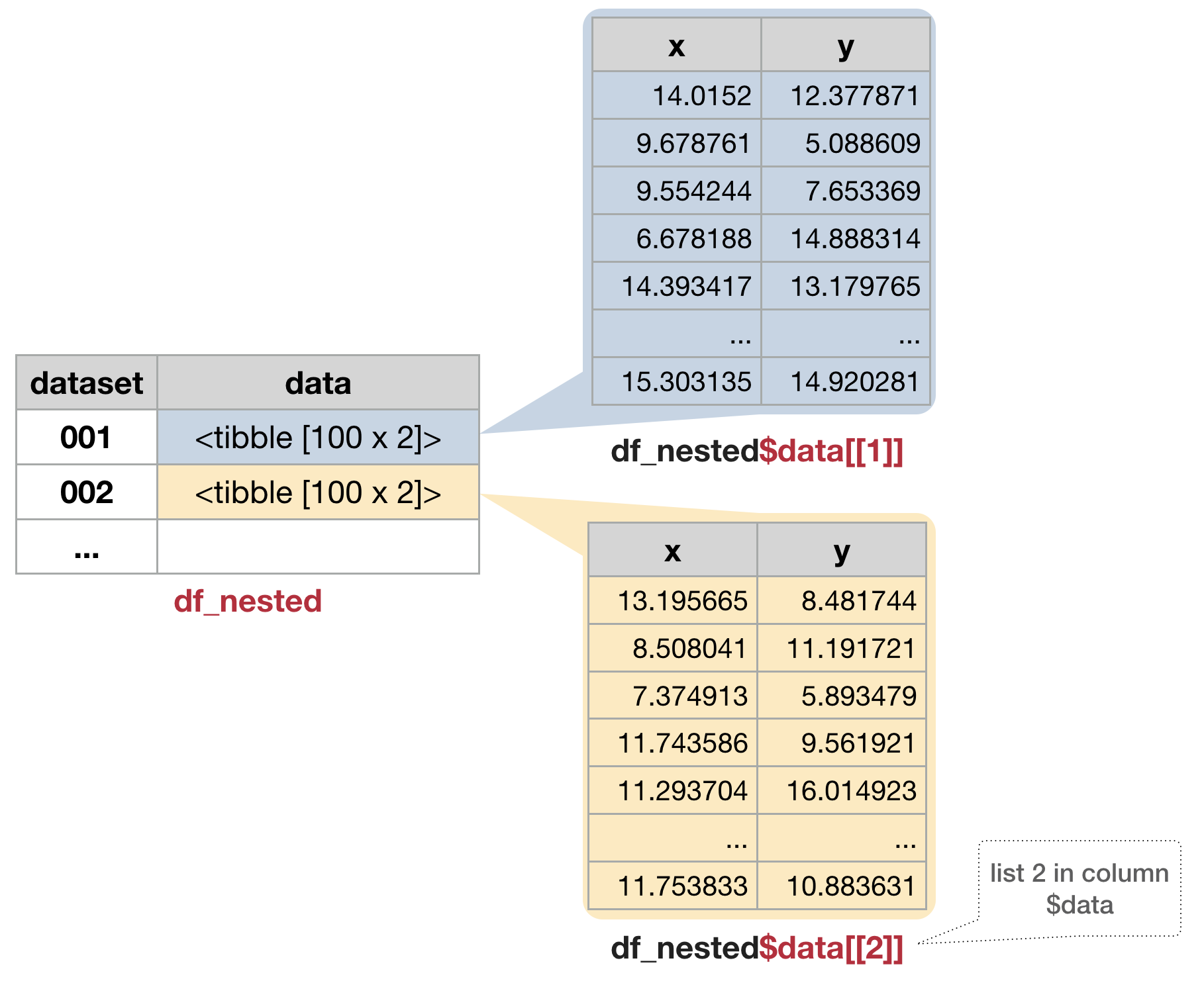
- Tibbles are particularly good in handling and visualizing list-columns:
## # A tibble: 100 x 2
##   dataset data
##   <chr>   <list>
## 1 1       <tibble [100 × 2]>
## 2 2       <tibble [100 × 2]>
## # … with 98 more rows
How to make a dataframe with list-columns
- Use
tidyr::nest()to create a nested dataframe in which individual tables are stored within the cells of a larger table. - Use a 2-step approach: first group the data, then create the nested data with one row per group level.
# First convert data list into a tibble
df <- data_list %>% bind_rows()
# 2-step approach
df_nested <- df %>%
  group_by(dataset) %>%
  nest()
Map data-frames to the modeling function
- Nested data frames are useful when you want to preserve the relationships between observations and subsets of data.
- You can manipulate many sub-tables at once with the purrr mapping functions and save results as list-column in the same dataset:
model_nested <- df_nested %>%
  mutate(model = map(data, ~lm(y ~ x, data = .))) %>%
  print(n = 2)
## # A tibble: 100 x 3
##   dataset data               model
##   <chr>   <list>             <list>
## 1 1       <tibble [100 × 2]> <S3: lm>
## 2 2       <tibble [100 × 2]> <S3: lm>
## # … with 98 more rows
Extract some summary statistics using piped operations
stats_nested <- model_nested %>%
  mutate(
    alpha = map(model, coef) %>% # returns list-column with intercept/slope vector
      map_dbl(~ .[1]), # extract first element of each vector (same as ~ .x[1])
    # alternatively, in one go:
    beta = map_dbl(model, ~ coef(.x)[2]),
    r_sq = map(model, summary) %>% map_dbl(~.$r.squared)
  ) %>%
  print(n = 2)
## # A tibble: 100 x 6
##   dataset data               model    alpha  beta  r_sq
##   <chr>   <list>             <list>   <dbl> <dbl> <dbl>
## 1 1       <tibble [100 × 2]> <S3: lm>  3.12 0.794 0.668
## 2 2       <tibble [100 × 2]> <S3: lm>  2.64 0.800 0.701
## # … with 98 more rows
Use map2() to make the predictions
predict_nested <- stats_nested %>%
  mutate(pred = map2(.x = model, .y = data, .f = predict)) %>%
  print(n = 2)
## # A tibble: 100 x 7
##   dataset data               model    alpha  beta  r_sq pred
##   <chr>   <list>             <list>   <dbl> <dbl> <dbl> <list>
## 1 1       <tibble [100 × 2]> <S3: lm>  3.12 0.794 0.668 <dbl [100]>
## 2 2       <tibble [100 × 2]> <S3: lm>  2.64 0.800 0.701 <dbl [100]>
## # … with 98 more rows
Visualize the predictions
→ You need to get out of the nested data structure: tidyr::unnest()
unnest()makes each element of the list its own row,- but the list-columns have to be either atomic vectors or data frames!
predict_unnested <- predict_nested %>%
  unnest(pred) %>%
  print(n = 2)
## # A tibble: 10,000 x 5
##   dataset alpha  beta  r_sq  pred
##   <chr>   <dbl> <dbl> <dbl> <dbl>
## 1 1        3.12 0.794 0.668  14.3
## 2 1        3.12 0.794 0.668  10.8
## # … with 9,998 more rows
- Each regular column is repeated one for each row in the nested list-column.
- Using only
predinunnest()will omit thedatalist-column!
Visualize the predictions
- You can also unnest multiple columns simultaneously:
predict_unnested <- predict_nested %>%
  unnest(data, pred) %>%
  print(n = 2)
## # A tibble: 10,000 x 7
##   dataset alpha  beta  r_sq  pred     x     y
##   <chr>   <dbl> <dbl> <dbl> <dbl> <dbl> <dbl>
## 1 1        3.12 0.794 0.668  14.3 14.0  12.4
## 2 1        3.12 0.794 0.668  10.8  9.68  5.09
## # … with 9,998 more rows
Note: :
The `model` list-column cannot be unnested since all elements in the list-columns must have the same length!Visualize the predictions
- Now that we have a regular tibble, we can plot the predictions.
predict_unnested %>%
  ggplot(aes(x, pred)) +
    geom_line(aes(group = dataset), alpha = 0.3) +
    geom_smooth(se = FALSE)

Your turn...
Example DATRAS data
- Restructure the dataset to create a nested data frame grouped by species.
- Apply purrr's mapping function to model the species CPUE as a function of latitude.
- Save the models and summary statistics in the same nested dataframe.
- Generate ggplots with the predicted CPUE ~ lat per species and save these in a list-column.
- Identify the species where the CPUE is best explained by latitude and look at the prediction plot.
Overview of functions you learned today
purrr functions:
map(), map_lgl(), map_int(), map_dbl(), map_chr()
set_names()
map2(), map2_lgl(), map2_int(), map2_dbl(), map2_chr()
pmap(), invoke_map(), invoke_map_dbl()
invoke(), lmap(), imap(), walk(), walk2(), pwalk()
tidyr functions:
nest(), unnest()
How do you feel now.....?
Totally confused?

purrr provides any more useful functions for handling lists; see for more information
- the cheatsheet
- chapter 21 on iterations in R for Data Science
- a good tutorial for purr is also available on this webpage: https://jennybc.github.io/purrr-tutorial/
Totally bored?

Then apply more of the map functions to your second case study!
Totally content?
Then go grab a coffee, lean back and enjoy the rest of the day...!

Thank You
For more information contact me: saskia.otto@uni-hamburg.de
http://www.researchgate.net/profile/Saskia_Otto
http://www.github.com/saskiaotto

This work is licensed under a
Creative Commons Attribution-ShareAlike 4.0 International License except for the
borrowed and mentioned with proper source: statements.
Image on title and end slide: Section of an infrared satallite image showing the Larsen C
ice shelf on the Antarctic
Peninsula - USGS/NASA Landsat:
A Crack of Light in the Polar Dark, Landsat 8 - TIRS, June 17, 2017
(under CC0 license)