


Data Analysis with R
3 - Data structures and basic calculations
Saskia A. Otto
Postdoctoral Researcher
Some recap on data structures
Data structures
Five data types most often used in data analysis:
| Dimensions | Homogeneous | Heterogeneous |
|---|---|---|
| 1d | Atomic vector | List |
| 2d | Matrix | Data frame |
| nd | Array |
Lists

Lists
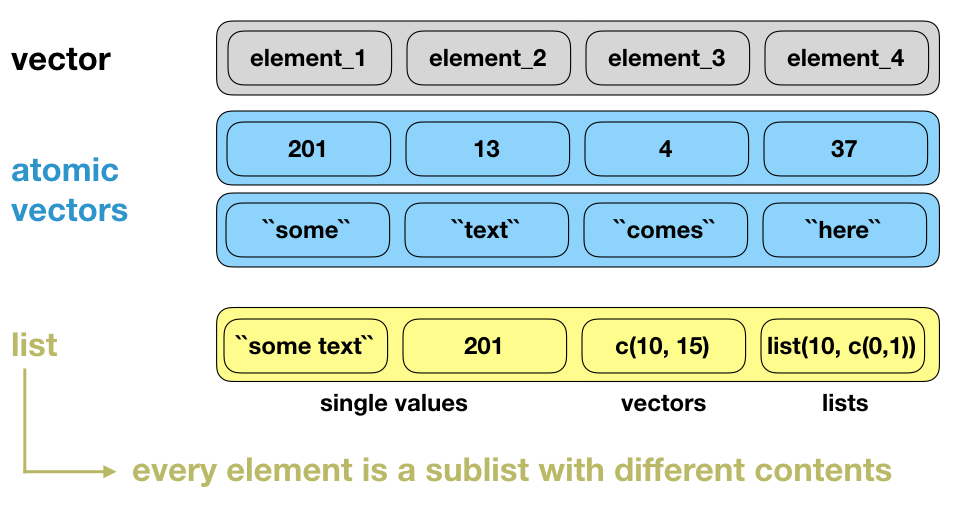
- are different from atomic vectors because their elements can be of any type, including lists
- you construct lists by using
list()instead ofc():
x <- list(1:3, "a", c(TRUE, FALSE, TRUE), c(2.3, 5.9))
str(x)
## List of 4
##  $ : int [1:3] 1 2 3
##  $ : chr "a"
##  $ : logi [1:3] TRUE FALSE TRUE
##  $ : num [1:2] 2.3 5.9
Lists are vectors
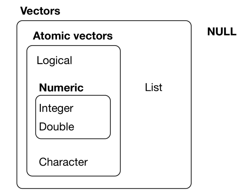
NULL is often used to represent the absence of a vector (as opposed to NA which is used to represent the absence of a value in a vector). NULL typically behaves like a vector of length 0.
Why is a list considered a vector?
Lists (cont)
- are sometimes called recursive vectors, because a list can contain other lists.
x <- list(list(list(list())))
str(x)
## List of 1
##  $ :List of 1
##   ..$ :List of 1
##   .. ..$ : list()
Visualization of the following lists
x1 <- list(c(1, 2), c(3, 4))
x2 <- list(list(1, 2), list(3, 4))
x3 <- list(1, list(2, list(3)))
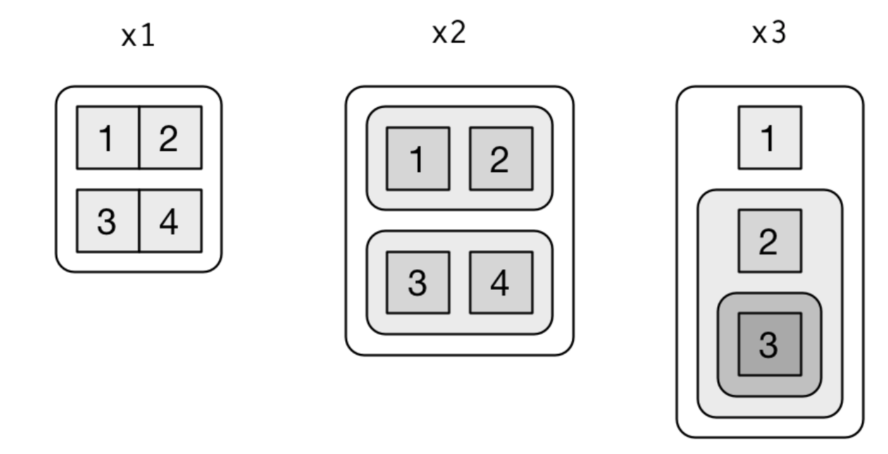
source: R for Data Science by Wickam & Grolemund, 2017 (licensed under CC-BY-NC-ND 3.0 US)
Lists (cont)
typeof()a list is a list- you can test for a list with
is.list()and - coerce to a list with
as.list() - you can turn a list into an atomic vector with
unlist(). - if the elements of a list have different types,
unlist()uses the same coercion rules asc(). - lists are used to build up many of the more complicated data structures in R.
Structure of lists
A very useful tool for working with lists is str() because it focuses on the structure, not the content.
x <- list(1, 2, 3)
str(x)
## List of 3
##  $ : num 1
##  $ : num 2
##  $ : num 3
Structure of lists
A very useful tool for working with lists is str() because it focuses on the structure, not the content.
x <- list(1, 2, 3)
str(x)
## List of 3
##  $ : num 1
##  $ : num 2
##  $ : num 3
x_named <- list(a = 1, b = 2, c = 3)
str(x_named)
## List of 3
##  $ a: num 1
##  $ b: num 2
##  $ c: num 3
Subsetting
Three ways to subset a list:
[extracts a sublist.[[extracts a single component from a list.$is a shorthand for extracting named elements of a list.
Subsetting (cont)
I will demonstrate each way using the following list:
a <- list(a = 1:3, b = "a string", c = pi, list(-1, -5))
str(a)
## List of 4
##  $ a: int [1:3] 1 2 3
##  $ b: chr "a string"
##  $ c: num 3.14
##  $  :List of 2
##   ..$ : num -1
##   ..$ : num -5
Subsetting: '[ ]'
1.[ extracts a sublist. The result will always be a list (it keeps the original list 'container' and removes all elements not selected). Like with vectors, you can subset with a logical, integer, or character vector.
str(a[1:2])
## List of 2
##  $ a: int [1:3] 1 2 3
##  $ b: chr "a string"
str(a[4])
## List of 1
##  $ :List of 2
##   ..$ : num -1
##   ..$ : num -5
a[4]
## [[1]]
## [[1]][[1]]
## [1] -1
##
## [[1]][[2]]
## [1] -5
Subsetting: '[[ ]]'
2.[[ extracts a single component from a list. It removes a level of hierarchy from the list (= you remove one 'container').
str(a[[1]])
## int [1:3] 1 2 3
str(a[[4]])
## List of 2
##  $ : num -1
##  $ : num -5
a[[4]]
## [[1]]
## [1] -1
##
## [[2]]
## [1] -5
Subsetting: '$'
3.$ is a shorthand for extracting named elements of a list. It works similarly to [[ except that you don’t need to use quotes.
a$a
## [1] 1 2 3
# same as
a[["a"]]
## [1] 1 2 3
Some visualization of subsetting lists
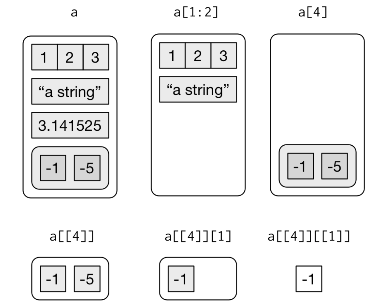
source: R for Data Science by Wickam & Grolemund, 2017 (licensed under CC-BY-NC-ND 3.0 US)
Your turn...
Visualize the following lists as nested sets
1. list(a, b, list(c, d), list(e, f))
2. list(list(list(list(list(list(a))))))
Quiz 1: Subsetting lists
The following list has been created:
list_example <- list(one = 1:10, two = letters,
  three = list(abc = c(132, 876, 42), xyz = c(T,F,F,T,F,T)), four = NULL)
What does the following return? list_example[1:2]
- a vector with the first 2 elements of each list
- a list of all sublists, each containing only the first 2 elements of the original sublists
- a list containing only sublist "one" and "two"
- NA
[ extracts always sublists and returns a list. In this example, you extract the first and second sublists, which are the numeric vector "one" and the character vector "two".
Quiz 2: Subsetting lists
The following list has been created:
list_example <- list(one = 1:10, two = letters,
  three = list(abc = c(132, 876, 42), xyz = c(T,F,F,T,F,T)), four = NULL)
What does the following return? list_example["four"]
- NULL
- error message
- a list containing NULL
- a vector with NULL elements
[ extracts always sublists and returns a list. In this example, you extract the sublist that is called "four", which is the fourth sublist containing NULL elements.
Quiz 3: Subsetting lists
The following list has been created:
list_example <- list(one = 1:10, two = letters,
  three = list(abc = c(132, 876, 42), xyz = c(T,F,F,T,F,T)), four = NULL)
What does the following return? list_example[[1]][2]
- a list containing "a"
- a list containing 1
- a vector containing "b"
- a vector containing 2
[[ extracts always single components from a list. In this case, it extracts the first sublist, which is a vector, and from there the 2nd element, which is a 2. So the returned object is also a vector containing only the number 2.
Quiz 4: Subsetting lists
The following list has been created:
list_example <- list(one = 1:10, two = letters,
  three = list(abc = c(132, 876, 42), xyz = c(T,F,F,T,F,T)), four = NULL)
What does the following return? list_example[3][[2]]
- NA
- a list containing FALSE
- the logical vector 'xyz'
- a vector containing "c"
- error message
This is a bit trickier! The code snippet tries to subset the following: return a list that extracts from 'list_example' the 3rd sublist and from this list take sublist 2.
BUT: that list has only 1 element, which is the list 'three' (containing vectors 'abc' and 'xyz'); a sublist 2 doesn't exist. However, the following would have worked: list_example[2:3][[2]] since now the extracted list contains 2 sublists, "two" and "three", from which it can subset list "three".
Quiz 5: Subsetting lists
What is equivalent to the following code (multiple answers correct)? And which of the options below returns a suprising value?
list_example[["three"]][c("abc", "xyz")]
- list_example[[3]][1:2]
- list_example[[3]][[1:2]]
- list_example[[3]][c("abc", "xyz")]
- list_example$three[1:2]
- list_example$three[c("abc", "xyz")]
Option 2 subsets something else, which is not so intuitive: it extracts also the 3rd sublist "three", but from there it subsets the 2nd element of the 1st sublist (the vector "abc"). DO NOT use this notation for extracting the number '876', use instead: list_example[[3]][[1]][2] (element 2 in sublist 1 within sublist 3)!!!
Quiz 6 - Challenge: Subsetting lists
Create a new vector that contains the 4th element of sublist "one" and element 1 and 3 from sublist "abc" within "three" in 'list_example'.
- What is the sum of this vector?
Within the vector you extract first the value from sublist "one" and then values from sublist "abc" within sublist "three" (both seperated by a comma).
To get the correct answer you could subset for instance like this:
sum( c(list_example[[1]][2], list_example[[3]][[1]][c(1,3)]) )
or using the $ sign:
sum( c(list_example$one[2], list_example$three$abc[c(1,3)]) )
- 176
Quiz 7 - Challenge: Subsetting lists
Execute the following R command in your console
lm_list <- lm(Sepal.Length ~ Sepal.Width, data = iris)
and look at the structure of the list you created with
str(lm_list, max.level = 1) # max.level=1 shows only the first level
# of the hierarchy (and not all sub/sub/..lists))
- What is the last value of the 'residuals'?
Look at the names of the sublists in lm_list. Is there anything that sounds like what we are looking for? If you found it check the number of elements it contains (we want the last one!).
The object created from a linear regression (that is what the lm() function does) is a long list with many nested lists. lm_list contains 12 sublists amongst one is a vector called 'residuals' (thats what we are after). So to get the last value (from the 150 values) type:
lm_list$residuals[150]
- 0.0438606
Other homogeneous data structures: matrices and arrays

Matrices and arrays
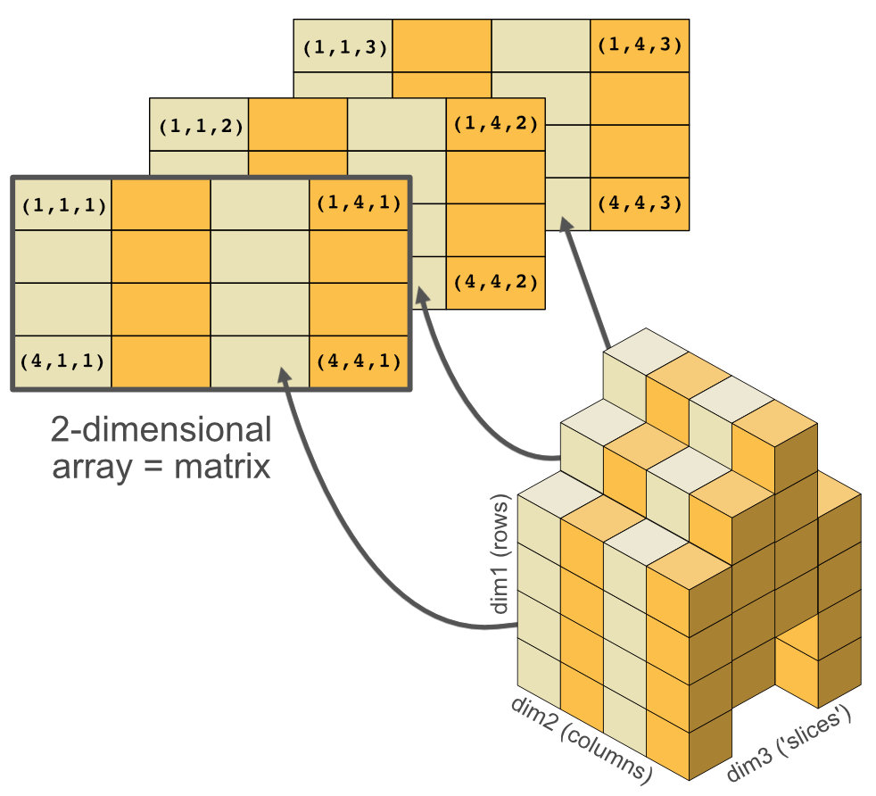
- Adding a
dimattribute to an atomic vector allows it to behave like a multi-dimensional array. - A special case of the array is the matrix, which has two dimensions.
- Matrices are used commonly as part of the mathematical machinery of statistics.
- Arrays are much rarer, but worth being aware of.
Creating matrices
Matrices are created with
matrix()- or by combining vectors (of equal length) to a matrix using
cbind()(stands for column-binding).
Creating matrices
Matrices are created with
matrix()- or by combining vectors (of equal length) to a matrix using
cbind()(stands for column-binding).
a <- matrix(1:6, ncol = 3, nrow = 2)
a
##      [,1] [,2] [,3]
## [1,]    1    3    5
## [2,]    2    4    6
v1 <- 1:3
v2 <- 4:6
a <- cbind(v1, v2)
a
##      v1 v2
## [1,]  1  4
## [2,]  2  5
## [3,]  3  6
Attributes length and names
length() and names() have high-dimensional generalisations:
Attribute length
length() generalises to
nrow()andncol()for matrices, anddim()for arrays.
length(a)
## [1] 6
nrow(a)
## [1] 3
ncol(a)
## [1] 2
Attribute names
names() generalises to
rownames()andcolnames()for matrices, anddimnames(), a list of character vectors, for arrays.
colnames(a) <- c("A","B")
rownames(a) <- c("a","b","c")
a
##   A B
## a 1 4
## b 2 5
## c 3 6
Subsetting matrices and arrays
Most common way of subsetting matrices (2d) and arrays (>2d) is a simple generalisation of 1d subsetting:
- You supply a 1d index for each dimension, separated by a comma (integer, logical, or character indices allowed).
- Blank subsetting is now useful because it lets you keep all rows or all columns.
a <- matrix(1:9, nrow = 3)
colnames(a) <- c("A", "B", "C")
a
##      A B C
## [1,] 1 4 7
## [2,] 2 5 8
## [3,] 3 6 9
a[1:2, 2]
a[, c("A", "C") ]
Guess which values you get!
Subsetting matrices and arrays
Most common way of subsetting matrices (2d) and arrays (>2d) is a simple generalisation of 1d subsetting:
- You supply a 1d index for each dimension, separated by a comma (integer, logical, or character indices allowed).
- Blank subsetting is now useful because it lets you keep all rows or all columns.
a <- matrix(1:9, nrow = 3)
colnames(a) <- c("A", "B", "C")
a
##      A B C
## [1,] 1 4 7
## [2,] 2 5 8
## [3,] 3 6 9
a[1:2, 2]
## [1] 4 5
a[, c("A", "C") ]
##      A C
## [1,] 1 7
## [2,] 2 8
## [3,] 3 9
Your turn...
Quiz 8: Subsetting matrices
Subset the following matrix...
(mat <- matrix(c(0,NA,4,18,35,97,7,9,20), nrow = 3))
##      [,1] [,2] [,3]
## [1,]    0   18    7
## [2,]   NA   35    9
## [3,]    4   97   20
to get all values in row 1
Submit and Compare ClearQuiz 9: Subsetting matrices
Subset the following matrix...
(mat <- matrix(c(0,NA,4,18,35,97,7,9,20), nrow = 3))
##      [,1] [,2] [,3]
## [1,]    0   18    7
## [2,]   NA   35    9
## [3,]    4   97   20
to get all values in row 1 and 3
Submit and Compare ClearQuiz 10: Subsetting matrices
Subset the following matrix...
(mat <- matrix(c(0,NA,4,18,35,97,7,9,20), nrow = 3))
##      [,1] [,2] [,3]
## [1,]    0   18    7
## [2,]   NA   35    9
## [3,]    4   97   20
to get all values in column 2
Submit and Compare ClearQuiz 11: Subsetting matrices
Subset the following matrix...
(mat <- matrix(c(0,NA,4,18,35,97,7,9,20), nrow = 3))
##      [,1] [,2] [,3]
## [1,]    0   18    7
## [2,]   NA   35    9
## [3,]    4   97   20
to get all values in row 2 and 3 and column 1 and 2
Submit and Compare ClearOther heterogeneous data structures: data frames

Data frames
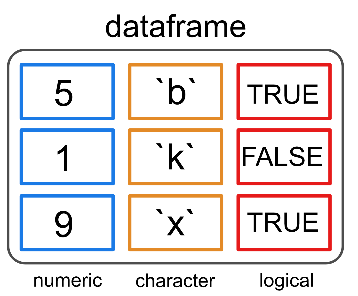
- Most common way of storing data in R.
- Represents a list of equal-length vectors
- → makes it 2-dimensional structure
- Shares properties of both the matrix and the list:
Data frames

- Most common way of storing data in R.
- Represents a list of equal-length vectors
- → makes it 2-dimensional structure
- Shares properties of both the matrix and the list:
- names: has
names(),colnames(), andrownames(), althoughnames()andcolnames()are the same thing. - length:
length()is the length of the underlying list and so is the same asncol();nrow()gives the number of rows.
- names: has
Generating data frames
You create a data frame using data.frame() (note the point inbetween both words!), which takes named vectors as input:
df <- data.frame(x = 1:3, y = c("a", "b", "c"))
str(df)
## 'data.frame':    3 obs. of  2 variables:
##  $ x: int  1 2 3
##  $ y: Factor w/ 3 levels "a","b","c": 1 2 3
- Beware of
data.frame()s default behaviour, which turns strings into factors. UsestringsAsFactors = FALSEto suppress this behaviour:
df <- data.frame(x = 1:3, y = c("a", "b", "c"), stringsAsFactors = FALSE)
str(df)
## 'data.frame':    3 obs. of  2 variables:
##  $ x: int  1 2 3
##  $ y: chr  "a" "b" "c"
Subsetting data frames
Either like a matrix (useful if several columns and rows are selected)
df[1:2, 1] # row 1-2, column 1
## [1] 1 2
Subsetting data frames
Either like a matrix (useful if several columns and rows are selected)
df[1:2, 1] # row 1-2, column 1
## [1] 1 2
Or like a list
df$x # shows all elements of column 'x'
## [1] 1 2 3
df$y[2] # 2nd element of column 'y'
## [1] "b"
df[[2]][2] # same
## [1] "b"
Your turn...
Generate a data frame yourself...
that contains
- 4 variables with differet data types (logical, character, double, and/or integer),
- all of length 20 and
- give each variable a name.
Quiz 12: iris dataset - data structure
Explore the following dataset
head(iris, 1)
##   Sepal.Length Sepal.Width Petal.Length Petal.Width Species
## 1          5.1         3.5          1.4         0.2  setosa
What type of data structure is iris?
- list
- matrix
- array
- data frame
Use the class() function to answer this question.
iris is a data frame because it is 2-dimensional and contains different types (it is heterogeneous).
Quiz 13: iris dataset - dimensions
What are the dimensions of the dataset iris?
- 5 rows, 150 columns
- 150 rows, 5 columns
Use the nrow() and ncol() functions to answer this question.
Quiz 14: iris dataset - data type
Which basic data types does the dataset iris contain?
- logical
- integer
- double
- character
- factor
- date
Use the str() function to answer this question.
The first 4 columns contain decimal numbers, the last is a character vector with additional attributes, which makes it a factor (see also attributes(iris$Species)).
Quiz 15: iris dataset - subsetting
- Calculate the sum of all observations in the dataset using the function
sum()
The easiest is to subset matrix-like within the sum function: sum( iris[, 1:4] )
- 2078.7
The workspace or the global environment

When you create R objects, you'll see them appear in your environment pane under Global Environment:
x <- 1:10
y <- 1:10
z <- cbind(x,y)  # matrix
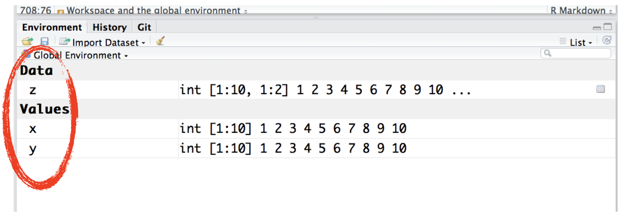
The global environment, more often known as the user's workspace, is the first item on the search path. When a user starts a new session in R, the R system creates a new environment for objects created during that session.
You can list all objects in the workspace using the function ls():
x <- 1:10
y <- 1:10
z <- cbind(x,y)  # matrix
ls()
## [1] "x" "y" "z"
Remove objects from workspace
You can remove an object with rm():
x <- 4
x
rm(x)
Remove objects from workspace
You can remove an object with rm():
x <- 4
x
rm(x)
Or remove all objects in one go:
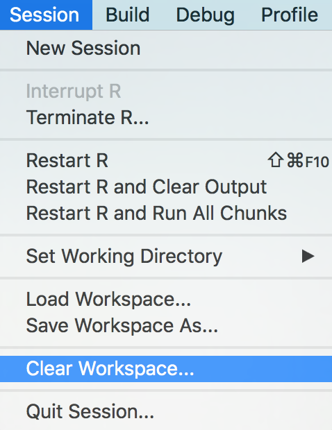
Overview of functions you learned today
str(), [, [[, $,
list, is.list(), as.list(), unlist(),
matrix(), cbind(), nrow(), ncol(), dim, rownames(), colnames(), dimnames(),
data.frame(), data.frame(stringsAsFactors = FALSE)
How do you feel now.....?
Totally confused?

Again, try out the online tutorial at Data Camp.
And go over this lecture again and do the quizzes.
Totally bored?

Then try out the following: Calculate for the iris data set
- the mean sepal and petal length per species, and
- the minimum petal width for the species "setose".
- Which species has the longest sepal width?
Totally content?
Then go grab a coffee, lean back and enjoy the rest of the day...!
Thank You
For more information contact me: saskia.otto@uni-hamburg.de
http://www.researchgate.net/profile/Saskia_Otto
http://www.github.com/saskiaotto

This work is licensed under a
Creative Commons Attribution-ShareAlike 4.0 International License except for the
borrowed and mentioned with proper source: statements.
Image on title and end slide: Section of an infrared satallite image showing the Larsen C
ice shelf on the Antarctic
Peninsula - USGS/NASA Landsat:
A Crack of Light in the Polar Dark, Landsat 8 - TIRS, June 17, 2017
(under CC0 license)