Case study 1:
Hydrographical dynamics in the Baltic Sea
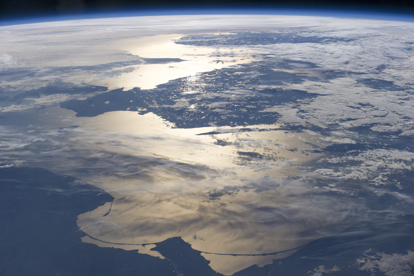
Foto: ISS Crew Earth Observations Facility and the Earth Science and Remote Sensing Unit, Johnson Space Center (under CC0)
Background
The Baltic Sea in Northern Europe is worldwide one of the greatest brackish water systems, extending over 13 degrees of latitude and thus featuring a strong temperature gradient across the different basins. Due to its semi-enclosed nature with a narrow connection to the North Sea, the Baltic Sea experiences a net positive freshwater balance. In the deep areas of the Central Baltic Sea, this leads to a permanent stratification with a highly saline deepwater (values > 12) being separated from low salinity surface waters (values < 9). Vertical mixing of the water masses is hence restricted by a halocline at about 60-100 m depth. The exchange of deepwater in these areas can only occur by strong pulses of salt water inflow. These so-called “major Baltic inflows” (MBI)1,2, can change the oceanological regime of the whole water column and improve the living conditions of for example benthic animals by the distribution of oxygenated water. During the summer months a thermocline develops at a depth of 20-30 m leading to an enhanced vertical habitat differentiation. Such stratifications create sub-habitats for fish and zooplankton species3,4,5
Over the past 3 decades we observed decreased frequencies of MBIs, which have been attributed to changed atmospheric forcing conditions. This resulted in decreased salinity levels due to the shallowing of the halocline affecting cod recruitment success and the zooplankton stock size of Pseudocalanus acuspes 6,7. After a 12-year stagnation period an MBI was recorded in January 2015, which brought highly saline waters into the Bornholm Basin (20 psu, according to Rak8).
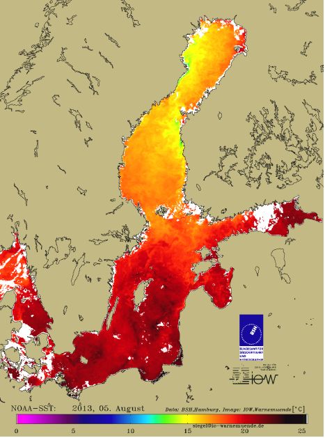
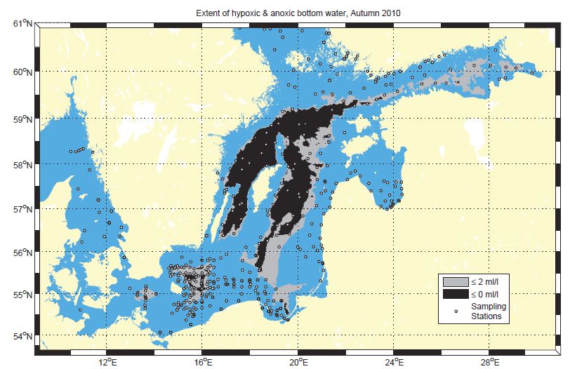
Maps: HELCOM environment fact sheets (under CC0)
Your task
This case study is meant to repeat all the single steps you learnt in the previous lectures and to summarize them into one analysis as you would do also with a real analysis. Some of the steps you probably will have done already with the previous exercises → then simply put them together in your RMarkdown file, this time adding a bit more text on why you did what.
You will explore the oceanographical datasets downloaded from the ICES data portal for the Baltic Sea and the year 2015. The dataset contains of 30012 rows and 11 columns. A brief description of each column follows:
| Field | Description |
|---|---|
| Cruise | 4-digit codes referring to the research vessel (e.g. 34AR represents the Finnish vessel ARANDA) |
| Station | 4-digit codes assigned to every station |
| Type | Type of measurement: B = bottle data |
| yyyy-mm-ddThh:mm | Date and time |
| Latitude [degrees_north] | Station coordinates: Latitude in decimal degrees |
| Longitude [degrees_east] | Station coordinates: Longitude in decimal degrees |
| Bot. Depth [m] | Bottom depth at station (in metre) |
| PRES [db] | Pressure of measurement depth, in decibar (equivalent to metre depth) |
| TEMP [deg C] | Water temperature at specific measurement depth, in degree Celcius |
| PSAL [psu] | Salinity at specific measurement depth, measured in unit of PSU (Practical Salinity Unit) |
| DOXY [ml/l] | Concentration of dissolved oxygen at specific measurement depth, in mililitre per litre |
The RMarkdown file
Create an HTML RMarkdown file with the Case study as the title (see above). You should have the following YAML header:
---
title: "Case study 1: Hydrographical dynamics in the Baltic Sea"
author: "Group letter and all (full) names of the group members"
date: "November 2017"
output:
  html_document:
    toc: yes
---
Take advantage of all the formatting options using Pandoc’s Markdown syntax, e.g. #, ##, ###, horizontal lines (with ***), etc. (see for more info the RMarkdown cheatsheet!)
All your text should be OUTSIDE the R code chunks, all the R code and some comments for yourself INSIDE these chunks.
Please follow these guidelines:
- Every step should be documented (use headers for this).
- Try to write in English.
- Inform the reader (which will be me in the first place) why you do certain steps (e.g. why do you not do anything about NAs or why you convert them into something else).
- Every result you compute should be summarised in your own words and interpreted (if it is not part of one of the questions than 2 or 3 sentences will be sufficient).
- If you have any question write them with the following highlight syntax:
<mark>Question: Your text....</mark>→ now you learned HTML coding :-)!
Step 1: Data wrangling
As you learned now, before you can do any data manipulation and visualization you need to get the data into R in a tidy format:
- Import file “1111473b.csv”.
- Check if the parsed formats for the variabeles are correct, check the date format.
- Rename the variables to something shorter following the R syntax guidelines.
- Make the data tidy:
- Is any restructuring needed?
- Is any separation or union needed?
- Are the data types correct?
- Do you need to handle NAs?
- Are there any awkward values in the data (potential typing errors)?
Before you can explore the dataset lets to some final data tidying in terms of the date: Create additional variables that contain only year, month, day, and yday (day-of-the-year), but keep the original date/time column.
Depending on the question of interest you need to transform and/or aggregate your dataset every time differently, e.g.
- you might need to aggregate over the different depth measurements if you are only interested in the sampling itself
- you might need to aggregate over the different depth measurements AND the samplings if you are only interested in the stations.
Remember, the dplyr package offers many functions for doing all kinds of data manipulations (the cheatsheet is really helpful)!
Step 2: Data quality check
(see also the exercises in lecture 7 - Data wrangling: 3.transformations)
- If you consider aggregating your data over different depth ranges (e.g. surface, mid-layer, deepwater) or if you want to filter certain depths you should be aware of
- the most frequently sampled depth and
- the most common depth profiles taken (Every 1 metre, every 5 metres?)
- If you want to aggregate your data over the months, you should be aware of
- the number of stations sampled → if unbalanced, a weighted mean might be more suitable?
- whether stations were sampled more than once in that month → should you calculate a station mean (aggregating the different samplings) first before you calculate a monthly mean? Would it make a difference? (Always try out the different versions and compare!)
- where there any temporal gap during the year where no sampling took place? → that might bias your monthly mean results
- If you want to exclude NAs or treat them in a specific way, it is good to know whether they occur randomly in your dataset or if there is a specific pattern
- are NAs in the dataset related to specific months or cruises? → maybe you want to consider excluding the entire cruise/month?
Step 3: Ecological questions
The following list of questions summarises mainly all the ideas you collected. I want you to investigate (numerically by looking at summarized data tables and graphically by producing different ggplots):
- Temporal components
- Can you find a seasonal pattern in the overall temperature, salinity, and oxygen conditions (for the complete Baltic Sea)?
- Is the seasonal dynamic everywhere the same or does it vary in different areas/basins?
- Spatial components (horizontally)
- Can you see in the data a spatial gradient of temperature, salinity, and oxygen conditions across the Baltic Sea?
- If there is a gradient, is it a continuous one or can you define certain areas that are similar?
- Are there any seasonal or monthly changes in the spatial pattern of these 3 parameters?
- Spatial components (vertically
- Can you identify a water stratification in terms of temperature, salinity, and oxygen conditions? For which parameters, which months and which areas?
- Comparison with findings of Rak (2016):
- If you select only stations that are close to the transect described in Figure 1 (i.e. stations around 55°N and between 15° and 19°E), do you find a similar vertical distribution of temperature, salinity, and oxygen for January and February?
- 2015 vs. 2014 (voluntarily):
- If you are interested to compare the depth profile from 2015 (after the MBI) with the time before (e.g. 2014) than download the data from ICES and apply the same steps to the data to make a comparison. Do you see and improvement in salinity and particularly oxygen conditions in the Central Baltic Sea in 2015?
References
Wyrtki, K. 1954. “Der Große Salzeinbruch in Die Ostee Im November Und Dezember 1951.” Kiel. Meeresforsch. 10, no. 1: 19-25.↩
Fonselius, S. H. 1969. “Hydrography of the Baltic Deep Basins Iii.” In Series Hydrography, 97: Fishery Board of Sweden↩
Otto, S.A., Diekmann, R., Flinkman J., Kornilovs G., and C. Möllmann. 2014. “Habitat Heterogeneity Determines Climate Impact on Zooplankton Community Structure and Dynamics.” PLoS ONE 9, no. 3: e90875.↩
Schaber, M., H. H. Hinrichsen, S. Neuenfeldt, and R. Voss. 2009. “Hydroacoustic Resolution of Small-Scale Vertical Distribution in Baltic Cod Gadus Morhua—Habitat Choice and Limits During Spawning.” Mar. Ecol. Prog. Ser. 377: 239-53.↩
Schulz, J., C. Möllmann, and H. J. Hirche. 2007. “Vertical Zonation of the Zooplankton Community in the Central Baltic Sea in Relation to Hydrographic Stratification as Revealed by Multivariate Discriminant Function and Canonical Analysis.” J. Mar. Syst. 67, no. 1-2: 47-58.↩
Möllmann, C., R. Diekmann, B. Müller-Karulis, G. Kornilovs, M. Plikshs, and P. Axe. 2009. “Reorganization of a Large Marine Ecosystem Due to Atmospheric and Anthropogenic Pressure: A Discontinuous Regime Shift in the Central Baltic Sea.” Glob. Change Biol. 15: 1377-93.↩
Otto, S.A., Kornilovs, G., Llope, M. and C. Möllmann. 2014. “Interactions among Density, Climate, and Food Web Effects Determine Long-Term Life Cycle Dynamics of a Key Copepod.” Mar. Ecol. Prog. Ser. 498: 73-84.↩
Rak, D. 2016. “The Inflow in the Baltic Proper as Recorded in January–February 2015.” Oceanologia 58, no. 3:241-47.↩